
|
|
|
|
|
Example 5.06:: 2R Planar: Joint Rates, Example 2 (MATLAB)
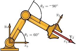
This example uses the inverse Jacobian to compute the joint rates for the 2R planar manipulator. It uses the 2  2 Jacobian resolved in the end-effector frame.
Contents
Clear All Workspace Objects and Reset All Assumptions
clear all
Structural Parameters
a1 = 30; % cm
a2 = 30; % cm
Given Joint Values
theta1 = 60; % deg
theta2 = -90; % deg
theta12 = theta1 + theta2; % deg
End-effector Linear Velocity Resolved in 
V2Res2 = [60; 0]; % [cm/s]
Inverse Jacobian: ![$[^{2}\overline\mathbf{J}_{2}]^{-1}$](Example05_06_eq19551.png)
detJ2Res2 = a1*a2*sind(theta2);
invJ2Res2 = (1/detJ2Res2)*[ a2,                      0;
                           -(a2 + a1*cosd(theta2)),  a1*sind(theta2)];
Joint Rates  in rad/s
ThetaDot = invJ2Res2*V2Res2 % [rad/s]
ThetaDot =

    -2
     2
Joint Rates in deg/s
ThetaDotDeg = (180/pi)*ThetaDot % [deg/s]
ThetaDotDeg =

 -114.5916
  114.5916
This MATLAB example illustrates a computation from the textbook Fundamentals of Robot Mechanics by G. L. Long, Quintus-Hyperion Press, 2015. See http://www.RobotMechanicsControl.info for additional relevant files.